Explanation of tracking macros

Part 1: Figure out how to identify particles

This depends on your raw data; in some cases your particles are easy to identify, in other cases you may even have to write special software to identify your special particles. (One person I talked to, I think it was Darren Link, wanted to track defects in liquid crystals, like the image to the right, for example. You'll have to figure out how to locate objects like that on your own.) Most people are trying to track particles that are fairly unambiguous.

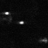
First, read in your image or stack of images. The kit includes the function readtiffstack, which can read in tiff stacks (click here for more information on this function). In the image below, we are looking at 2 micron diameter fluorescent particles using a confocal microscope. The array in this example is 100 x 100 pixels by 1500 images, perhaps 50 seconds of data taken at 30 frames per second.

IDL> a = readtiffstack('filename.tif') IDL> a0 = a(*,*,0) IDL> tvscl,a0 IDL> help,a,a0 A BYTE = Array[100, 100, 1500] A0 BYTE = Array[100, 100]

The particles that interest you should be between 5 and 20 pixels in diameter, ideally. The software is designed to look for bright particles on a black background, as in the above image. I like to make a copy of the first slice of the array (called "a0" in this example) to work with, rather than the whole array.

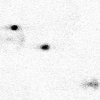
If you have black particles on a bright background, you'll have to invert the image before further processing:

IDL> temp = 255b-a0 IDL> tvscl,temp (You wouldn't normally want to invert the fluorescent image we're using as the example.)

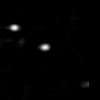
The software likes 'gaussian-like' blobs on a zero (black) background. So, filter the image to make it look like that...

IDL> b=bpass(a0,1,11) IDL> tvscl,b

bpass is a spatial bandpass filter which smooths the image and subtracts the background off. The two numbers are the spatial wavelength cutoffs in pixels. The first one is almost always '1'. The second number should be something like the diameter of the 'blob's you want to find in pixels. Try a few values and use the one that gives you nice, sharply peaked circular blobs where your particles were; remember the numbers you used for bpass. You can use the built-in function profiles to check with a cursor the size of your particles in your original image to help choose the upper cutoff for bpass.

Next, find the coordinates of the features. The parameter (11) is the diameter of the particles; typically it is the same as your bpass upper cutoff.

IDL> f = feature(b,11)

% FEATURE:  49 features found.

F               FLOAT     = Array[5, 49]

This will find a lot of possible particles in the image, you need to figure out how to select just the ones you want. John Crocker intentionally made 'feature' very sensitive, so it would never ignore something you were interested. You have to tell it what to ignore.

Examine the coordinates:

IDL> print, f(*,0:2)

9.59703      2.34431      215.181      7.23739     0.230804
24.6682      2.49346      607.877      9.93362     0.114143
38.1040      2.04013      98.8441      4.36558     0.294717

f consists of 5 columns of data, one 'row' for each particle in the image. The numbers are (1) x-centroid (2) y-centroid (3) total brightness (4) radius of gyration and (5) 'eccentricity' which is 0 for circles and 1 for lines. You will be most interested in the x and y coordinates, of course, but the other data allow you to 'discriminate' wanted from unwanted particles. Please read our comment about the radius.

You can also compare your original image with where the particles were found:

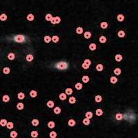
IDL> fo=fover2d(a0,f,/big)

This plots dots where each particle was found. On some computers the dots will be a red color, others will have white dots. The option /big doubles the size of the picture to make it easier to see, although if your original image is already 640x480 you shouldn't need to do this. The function fover2d returns an image. So, look at the red dots on top of your image, see that you found the guys that you wanted and guys you didn't.

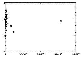
Next we want to discriminate the particles by size and brightness.

IDL> plot,f(2,*),f(3,*),psym=6 The horizontal axis is brightness, the vertical is radius of gyration. In general the brightest particles are the ones you want; in this particular case you see two distinct dots at the right, and the dots at the left are just due to random noise in your starting image.

Decide on a value on the x-axis that divides the two clouds of particles. For this case, a value of 10000 should work. This is the 'masscut' which you can use as a parameter to feature. Now, refind the particles, using this 'masscut' to reject false particles:

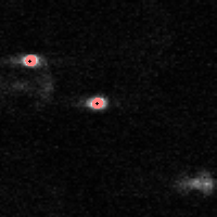
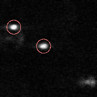
IDL> f = feature(b,11,masscut=10000) % FEATURE: 2 features found. IDL> fo=fover2d(a0,f,/big) IDL> fo2=fover2d(a0,f,/big,/circle,radius=15) IDL> flick, big(a0),fo2 The first fover2d command is at left, the second at right. Often it is useful to compare the fover2d image with the raw image, using the flick command. (Click here to download big.pro.)

Now there should be dots only on real particles. If not, you will need to modify the masscut, manually cut out particles based on size or eccentricity, or even start over re-imaging the system in a cleaner way.

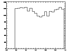
Next, test for pixel-biasing. For our sample image, we only have two particles, so we can't really check for pixel biasing (although it can be done at a later step for this data, see Part 2 below). Suppose you have a lot of particles from your test image...

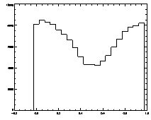
IDL> plot_hist,f(0,*) mod 1 The histogram at left looks the way we want it to look, mostly flat. The one on the right is not that great, with a deep dip in the middle.

One failure mode is if the length scale in feature is made too small, then all the x and y coords get 'rounded off' to the nearest pixel value. The above command plots a histogram of the fractional part of the x-coords of the image. The physically distributed positions should be random -- giving a flat histogram. If the histogram has two peaks (near 0 and 1), set the size parameter in 'feature' a little bigger, determine a new masscut, and repeat until everything is happy.

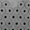
This assumes, of course, that you want to locate your particles with subpixel accuracy. Eric once tracked the particles you see at the right, a bunch of disks that have been painted by hand with dots. The accuracy of the position of the paint is not to within a pixel, so it's not worth worrying about getting subpixel accuracy for these types of images.

Note that plot_hist is part of our tracking kit.

Congratulations! You've done about 90% of what you have to do.

We have a procedure to do this for you, epretrack. It lets you set all of the parameters you need. (Follow the link to get more information.) You can apply this procedure to many files at once; the files can be movies or single images. You should read it over to see what it is doing.

The goal of epretrack is to create one file of coordinates 'pt.fname' for every original movie file. Run epretrack:

IDL> epretrack,'demo',bplo=1,bphi=11,dia=11,mass=10000,/tiff,/multi

Then, read in one of the pt files that contains the pre-tracked data.

IDL> pt=read_gdf('pt.demo.gdf')
IDL> help,pt

PT              FLOAT     = Array[6, 22545]

The files contain data for many particles in many different frames. To keep track of which frame a particle was found, an additional 'time' column is added to the data (read a file and see if it makes sense). That is, the coordinates for each frame are just 'concatenated vertically', with a time label (pt(5,*)). If you want to track a time interval longer that the length of a single movie, you should write something which 'concatenates' multiple 'pt' files together into a single array. You will have to fix the 'time column' such that it is monotonically increasing. (You can try catptdata2.pro, documentation coming at some point.)

Then you want to check how it all worked:

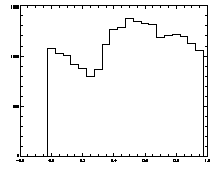
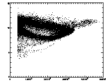
IDL> plot_hist,pt(0,*) mod 1 IDL> plot,pt(2,*),pt(3,*),psym=3 The first plot is at left, the second at right.

The second command checks the pixel biasing as discussed above (which seems OK); the third command verifies that you have a nice cloud of data in the brightness-radius space. If you have two or more clouds, figure out which cloud is for particles and which ones are artifacts, then either rerun epretrack with different parameters, or get rid of the data using some other method.

In the example shown above, the cloud has structure. This is mainly due to the microscopy and spherical aberation. Particles out of focus appear as distorted donuts. The distortion is different for particles above or below the field of view; thus particles slightly out of focus have distinctive total brightness and size. The sideways "U" seen in the plot above shows this: the rightmost part of the dense "U" is for in-focus particles, and the two branches pointing to the left are for particles above/below the focus. If you're not dealing with a system with this sort of problem, you should get a much more compact cloud.

There are also some particles with smaller than average radius; these are probably particles clipped at the edge of the field of view. The images started being 256 x 240 pixels; because of bpass, particles cannot be found in a 10-pixel margin around the edge (as our bpass parameter was 11). However, particles too close to the edge get clipped. We want to remove these from the data.

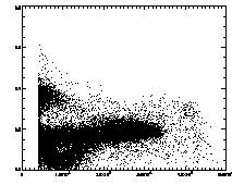
Further, we can plot the eccentricity -vs- brightness:

IDL> plot,pt(2,*),pt(4,*),psym=3 The particles with eccentricity larger than about 0.28 are low-brightness, and long and skinny (recall 0 eccentricity is for circles, 1 is for lines). A few of these large eccentricity particles are again due to being at the edge, and many are due to the spherical aberation problem. (The aberation especially causes problems when a single particle appears as a large donut shape, and two parts of the donut are grabbed as two semicircular shaped particles.)

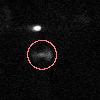
So, suppose we have gotten rid of these particles -- either by using where, changing the epretrack parameters, or improving the imaging. You may find fover2d useful; you can select some "bad" particles from the pretracked data using where, then fover2d them with your movie file, then run the resulting movie to see what in your images are registering as those "bad" particles:

IDL> a=read_gdf('demo.gdf') IDL> pt=read_gdf('pt.demo.gdf') IDL> w=where(pt(4,*) gt 0.3) IDL> fo=fover2d(a,pt(*,w),/circle,rad=15) IDL> movie,fo One of the "bad" particles is circled at left. (Then again, you might decide that for your purposes this is a "good" particle.)

So, let's suppose you've gotten rid of the bad particles. Your data may now look more like this:

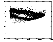
IDL> ptb=read_gdf('pt.demo2.gdf') IDL> plot,ptb(2,*),ptb(3,*),psym=3 IDL> plot,ptb(2,*),ptb(4,*),psym=3 The first plot is at left, the second at right.

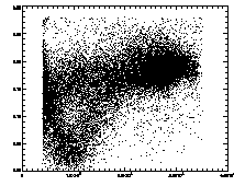
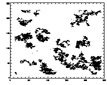
If you read in one of these files and: IDL> plot,ptb(0,*),ptb(1,*),psym=3 you should see lil clouds or streaks where the particles are.

In case you're curious, you can inspect the two demonstration pretrack files yourself, download the zip file below. Or, one person reported problems with the GDF files, so just in case we have also provided text files and a text reader. (I checked the GDF files and they seem to work, but it may be platform-dependent.)

• zip file containing pt.demo.gdf and pt.demo2.gdf
• pt.demo.txt
• pt.demo2.txt
• readtext.pro (download and rename as readtext.pro)
  To use readtext: a=readtext('pt.demo.txt')
• write_text.pro -- just in case you'd like this too. (Download and rename as write_text.pro.)
• Some documentation on how to use write_text and readtext

Part 3: Link particles found in each frame together to form trajectories

IDL> ptb = read_gdf('pt.demo2.gdf')
IDL> t = track(ptb,5,goodenough=10,memory=5)
IDL> help,t

T               FLOAT     = Array[7, 19333]

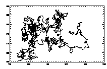
The output 't' is a 2D array. The first five columns are from feature (x,y,brightness,radius,eccentricity), the sixth column is the timestamp (from epretrack), and the seventh column is a unique particle ID#. Thus:

IDL> w=where(t(6,*) eq 7) IDL> plot,t(0,w),t(1,w),/isotropic,/ynozero or this will do the same thing: IDL> plotx,t,7,/x,/y

is the trajectory for particle #7. To see all of the trajectories:

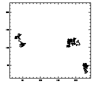
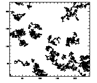
IDL> plottr,t IDL> plottr,t,goodenough=1 The first plot is at left, the second at right. The default is to plot only trajectories that are tracked for the complete time... so you can set goodenough to a small value, to plot all trajectories that last at least that duration.

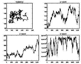
Another useful command for looking at lots of trajectories is: IDL> seeall,t enter=continue, ctrl-d=end 7 (size 1281) : You can keep hitting <enter> to see all of your trajectories, longest duration first. The z-coordinate in this case is the brightness (fluctuating as the particle goes in and out of focus slightly).

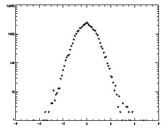
So what are all those intriguing options for track? Well, this is all well-documented in track's header comments. But I'll mention some important ones here. The first number is a displacement: what is the maximum distance you expect a particle will move between frames? The tracker will search for particles within that distance. I like to check this after the fact by making a histogram of the displacements between successive frames.

IDL> t = track(ptb,5,good=10,memory=5) IDL> plot_hist,mkpdf(t,1),/log If the histogram dies gracefully to zero before you get to your maximum displacement (in this case 5), you're doing great. mkpdf is a function which returns all of the displacements (both dx and dy) for a given dt, in this case, 1.

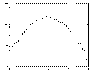
IDL> t2 = track(ptb,2,good=10,memory=5) IDL> plot_hist,mkpdf(t2,1),/log If you see an abrupt truncation at your maximum displacement (set now to 2), you're in trouble. Note that the bins at the edge of the histogram still have more than 20 points in each of them (the vertical axis goes from 10 to 10000, not from 1 to 10000 like the previous case).

We have other options: goodenough=10, memory=5. "goodenough" specifies the minimum duration for trajectories; particles tracked for less than ten frames are thrown away. This is helpful in case you have noise which occasionally appears as a particle, or particles that wander in and out of your field of view. "memory" allows you to track particles which temporarily disappear -- it acts as a memory. Thus particles may be missing for up to 5 frames in a row, but if they reappear in the same location, they are still considered the same particle. This can be useful if your particles are occasionally coming in and out of focus. If you're tracking a system where you always see all of your particles, set memory=0.

Check the header of the track.pro file for more information on the options.

Part 4: Analyze trajectories to do your science

We do have some additional tools which you may find useful which are posted here.

Contact us

• John Crocker: jcrocker(at)seas.upenn.edu
• Eric Weeks: weeks(at)physics.emory.edu