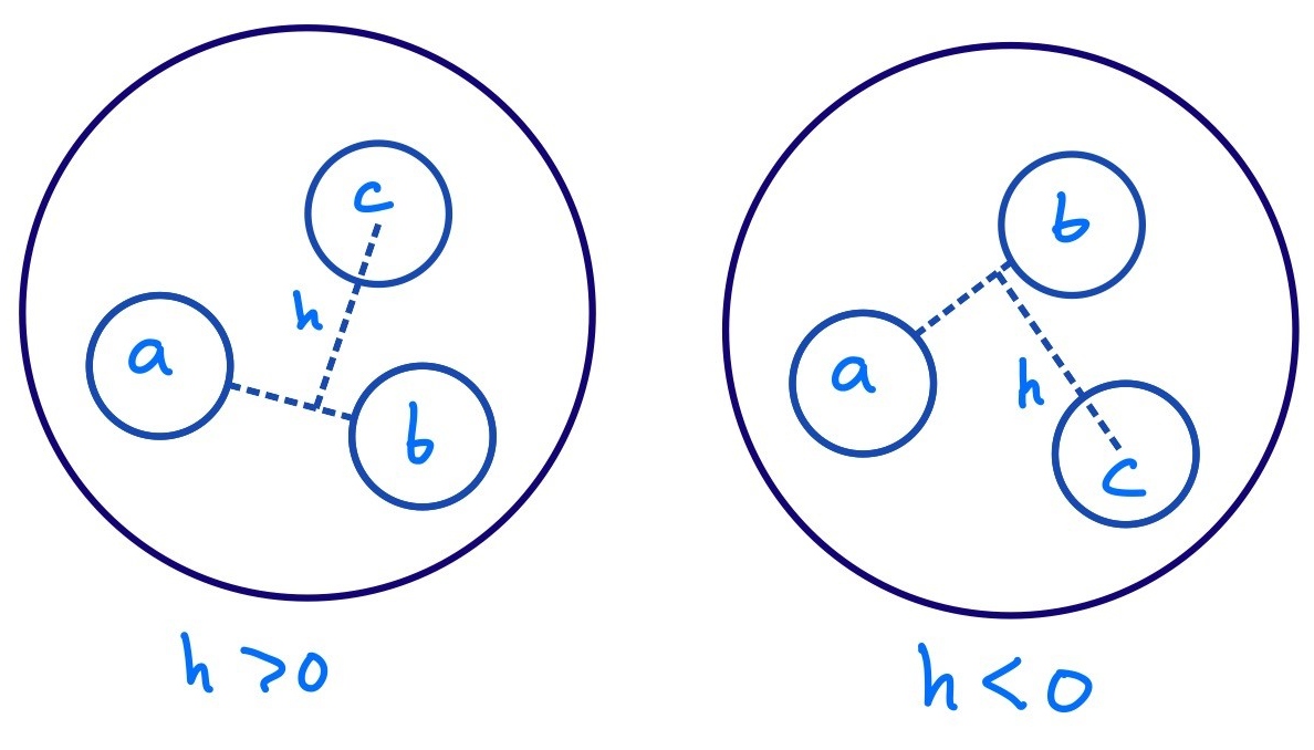
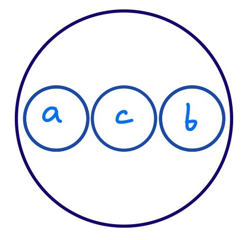
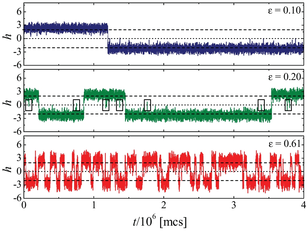
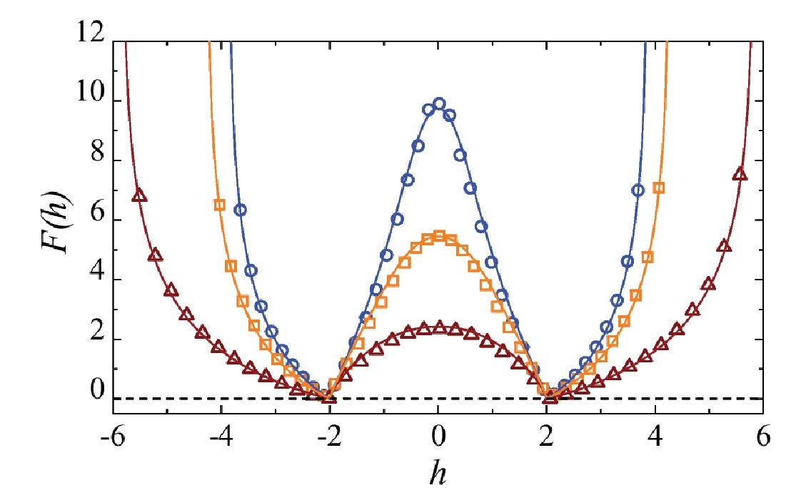
- "Free energy landscape for cage breaking of three
hard disks"
GL Hunter & ER Weeks, Phys. Rev. E 85, 031504 (2012).-
Abstract /
PDF /
arXiv:1112.5128 /
journal
- "Energy barriers, entropy barriers, and non-Arrhenius
behavior in a minimal glassy model"
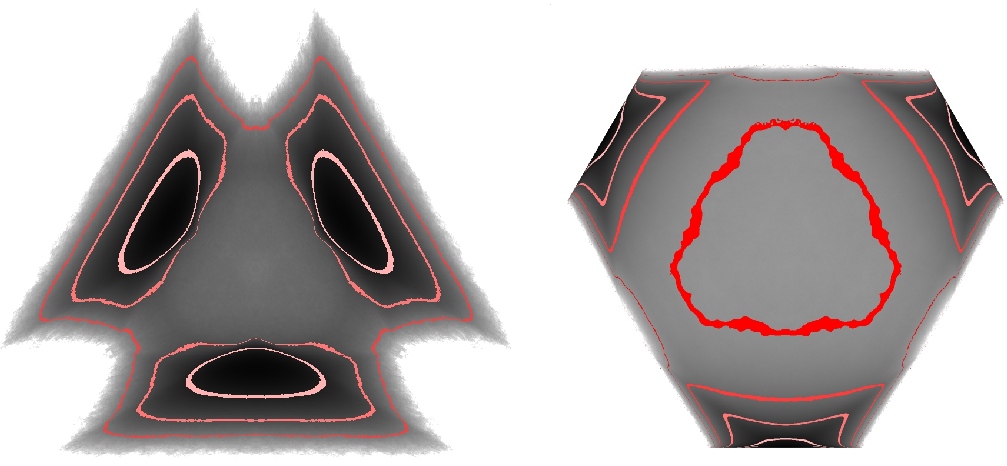
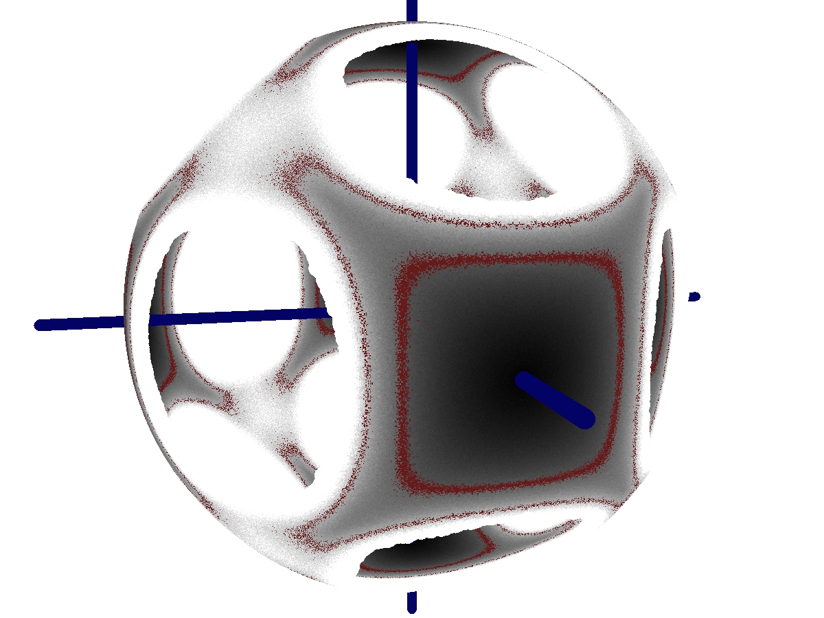
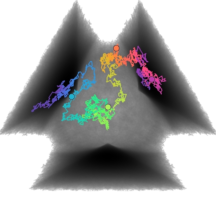
X Du & ER Weeks, Phys. Rev. E. 93, 062613 (2016) - "Visualizing free energy landscapes for four hard
disks"
ER Weeks & K Criddle, Phys. Rev. E 102, 062153 (2020)- Abstract / PDF / journal / arXiv:2001.11635v2 / download our data
- Simons webinar Eric gave about this work (March 24, 2021)
- Gary Hunter's PhD dissertation -- chapter 4 in particular
- Xin Du's PhD dissertation -- chapters 2 and 3 in particular
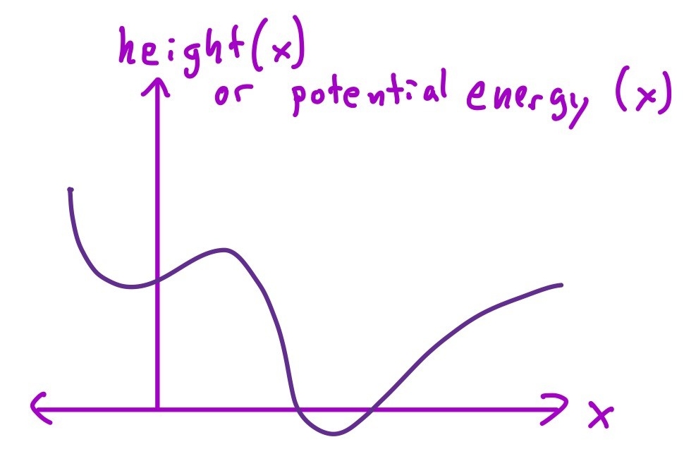
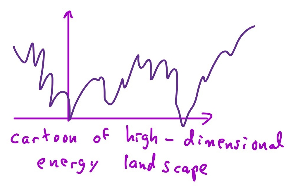
The paper by Weeks & Criddle is the most pedagogical of all of these, it's probably the best paper to start with.