Data from Figs. 5 and 6: fig5.txt, fig6.txt. Format of data: text file with 15 columns, 400 rows, corresponding to the trajectories shown in Figs. 5 and 6. Columns 1-8 are (x1,y1,x2,y2,x3,y3,x4,y4): the real-space coordinates. Columns 9, 10 correspond to (d1,d2) plotted in panel (g). Columns 11-13 are (c1,c2,c3) plotted in panel (f). Columns 14-15 are (u1,u2) plotted in panel (h). The locations marked by (b,c,d,e) in Fig. 5 correspond to rows 1, 331, 371, and 554 in the fig5 data. The locations marked by (b,c,d,e) in Fig. 6 correspond to rows 1, 101, 201, and 400 in the fig6 data.
Data from Fig. 7: fig7a-ep03.txt, fig7b-ep02.txt, fig7c-ep01.txt. Format of data: text file, columns = (time, raw c1, smoothed c1). The data plotted in the paper are smoothed over a time window of 10 tau_B, which corresponds to 100, 500, and 10 data points (as the raw data were sampled differently).
Data from Fig. 8: fig8.txt. Format of data: text file, columns = (epsilon, tau, 0 or 1). The third column is 0 for diffusive dynamics (blue circles in Fig. 8) or 1 for ballistic dynamics (red triangles in Fig. 8).
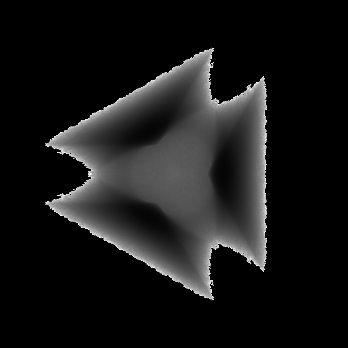
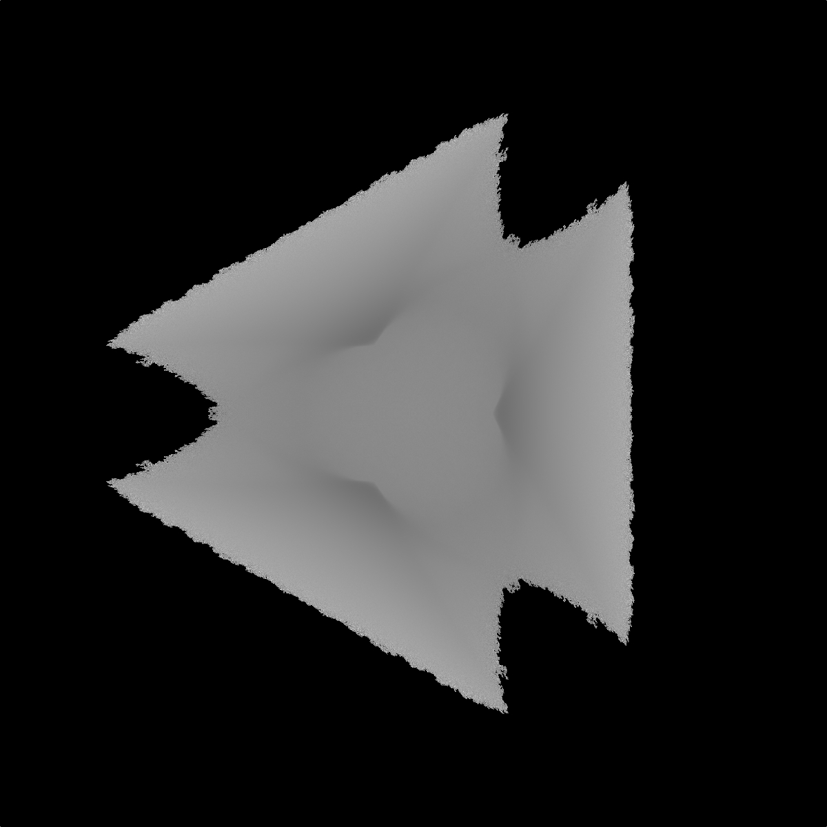
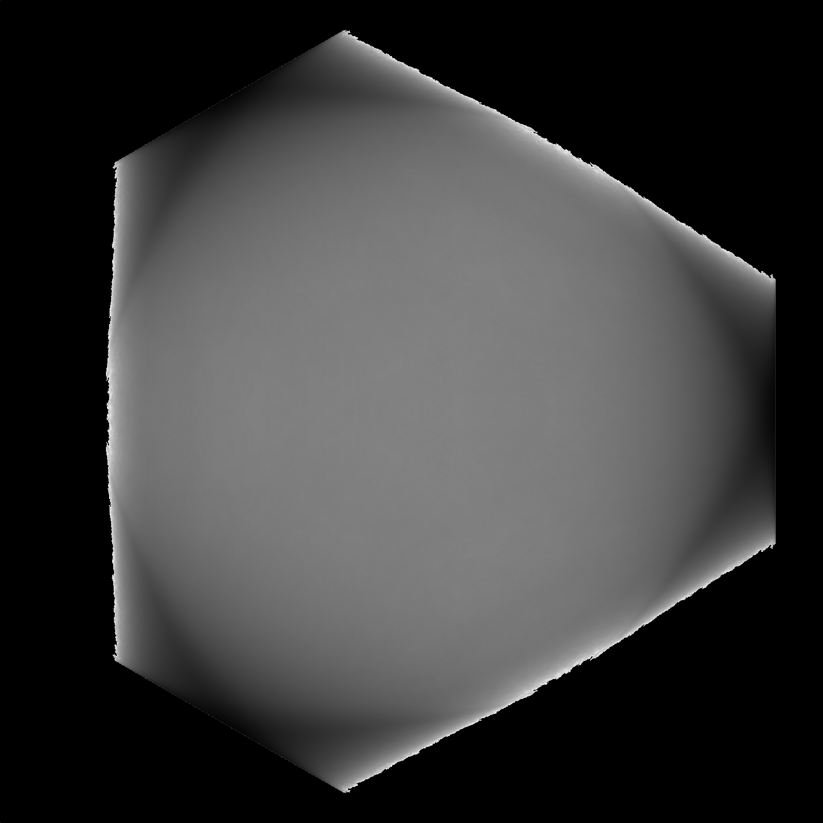
Data from Fig. 9: fig9.txt. Text file, 4 columns = (x,y,z,F) where F is the free energy. The minimum free energy is -7.11, the maximum is 0. As usual, the points with maximum free energy are nearly all at the edges of the phase space (the borders of the "holes" that correspond to cube edges). Note that the (x,y,z) points are not sampled uniformly over the sphere, in part because there's no straightforward way to do that. Rather, the points are generated on the surface of a cube and projected down to a unit sphere. For that matter, the original histogram of Omega is done based on a cubical surface. We first find the coordinates (c1,c2,c3) and then, knowing that this is symmetric, consider the coordinates in the first octant (all positive values). We then note further symmetry and project the points onto one face of a cube, so that Omega can be compiled in a 2D array with square histogram bins. It is this data that then gets turned back into a spherical projection. In the paper, when discussing barrier heights, we account for the fact that the square bins on the cube face become unevenly sized bins in the spherical phase space (which is what we really care about). That is, the same number of counts in a bin that's actually narrower in size sould be counted as a larger value of Omega than those counts in a bin that is wider. One more related data file: fig6f.txt: same thing, but for the 3D free-energy landscape of Fig. 6(f). The minimum free energy is -8.32, the maximum is -0.01.
Data from Fig. 10: PGM-formatted images, with contrast stretched. JPEG versions are provided, with quality set to 100%, although nonetheless JPEG compression has changed some of the pixel intensities by +/- 1. So for maximum quality, I recommend using the PGM images if you care about this from a data standpoint rather than merely wanting a qualitatively correct image.
Data from Fig. 11: fig11.txt. Format of data: text file, columns = (epsilon, u-height [green diamonds], c-height [red squares], d-height [purple triangles], log(tau) [filled blue circles]). The terms in [] describe the symbols of Fig. 11. The heights are the free energy barrier heights for the landscapes based on the u, c, and d variables.
Trajectory data: The trajectory data are in the format [x1,y1,x2,y2,x3,y3,x4,y4]. Note this format differs from almost all of our other track arrays available on the Weeks lab data pages. These files are small pieces of the simulation files, some of which would be larger than 100 MB. Note also that when we calculated the free energy landscapes by compiling the microstate counts (Omega), we did this from every single time step simulated. In contrast, these trajectories aren't saved every single time step, but rather every dN time steps (for the diffusive data).
For the ballistic data trajectory files, the data are spaced every 0.01 time increments. The particles are defined to have an initial velocity of 1.0, so that v1^2 + v2^2 + v3^2 + v4^2 = 4.0 holds true for all times due to conservation of kinetic energy. Thus if one takes the displacements from one line of data to the next, and divides by 0.01 to convert to velocity, this relation is essentially true (with the exceptions being times when a collision occurs, so that the displacement is not v*dt.) The units of length are in terms of particle radius (R = 1).
| filename | epsilon | data saved every dN steps | dynamics |
|---|---|---|---|
| traj-ep10j.txt (in a zip file) | 1.0 | 1000 | diffusive |
| traj-ep04j.txt (in a zip file) | 0.4 | 10000 | diffusive |
| traj-ep02j.txt (in a zip file) | 0.2 | 10000 | diffusive |
| traj-ep01j.txt (in a zip file) | 0.1 | 20000 | diffusive |
| traj-ep10p.txt (in a zip file) | 1.0 | n/a | ballistic |
| traj-ep05p.txt (in a zip file) | 0.5 | n/a | ballistic |
| traj-ep03p.txt (in a zip file) | 0.3 | n/a | ballistic |
| traj-ep02p.txt (in a zip file) | 0.2 | n/a | ballistic |
More ballistic data: The files above are trajectory files. These files below list the collisions that have occured, from which one can reconstruct trajectories at any temporal resolution you wish. These are again text files, with 18 columns of data: [x1, y1, vx1, vy1, x2, y2, vx2, vy2, x3, y3, vx3, vy3, x4, y4, vx4, vy4, C, time]. The first 16 columns are the positions and velocities of each particle right before a collision occurs. Given that the collision is at this moment, either two particles will be in contact (separation distance = 2) or one particle will be in contact with the outer wall. The data "C" indicates which collision is happening. C = [0,1,2,3] indicates that disk [0,1,2,3] is colliding with the wall. C = [4,5,6,7,8,9] indicates collisions between two disks: respectively 0+1, 0+2, 0+3, 1+2, 1+3, or 2+3. There's nothing really that useful about the variable C, I just included it for debugging purposes.