motion.pro
rm_motion.pro
(motion.pro revised 6/13/05)
NOTE: You also need getdx.pro
Often your data drifts; for example, your microscope stage may have hysteresis, or there may be some large-scale flow that you don't care about. These two programs help you diagnose & solve such problems.
You start with tracked data:
IDL> help,tra
tra FLOAT = Array[7, 505887]IDL> mot=motion(tra)
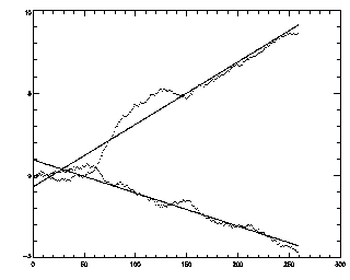
This generates the following plot:

One of these curves is the drift in the x-direction; the other is the drift in the y-direction. The dotted wiggly lines are the actual drift at every time step, and the straight lines are just linear fits to guide the eye. The way the drift is found is by examining the average dx and dy for each frame to the next frame; it only calculates the average over the particles which were tracked for both frames. The curves plotted are the integral of these measurements. (The raw data returned in the 'mot' array is only the dx's and dy's at each time. mot(0,*) is the time stamp, mot(2:3,*) are the dx's and dy's, mot(1,*) is sqrt(dx^2+dy^2), sort of a measure of the amount of motion occuring at that time.)
To get rid of the drift, call the next program:
IDL> trb=rm_motion(tra,mot)
This generates the same plot as above, to show you what it's done. In some cases you may notice that the sample doesn't move at a constant rate in time; you can adjust this with the "smooth" parameter, which will smooth the drift motion and then subtract the smoothed curve:
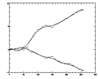 | IDL> trb=rm_motion(tra,mot,smooth=50) |
You should experiment with the smooth parameter to see what looks appropriate for your data. If you use smooth=1, you will subtract off all of your drift, which might be good if your sample was kicked abruptly at some point (although in general low values of smooth will overcompensate for small fluctuations in your data).
One way to check your data is to plot the trajectories, before and after the de-drifting:
IDL> plottr,tra,good=30
IDL> mot=motion(tra)
IDL> trb=rm_motion(tra,mot)
IDL> plottr,trb,good=30
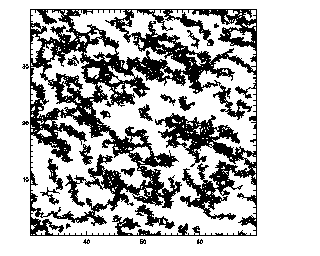
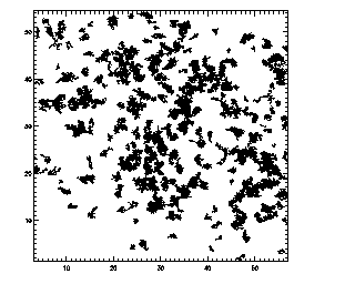
This was data where I artificially added in a linear drift in both x and y; the left picture shows how the data would look with the artificial drift, and the right picture shows how the trajectories look in the correct de-drifted reference frame. That is, when you have removed any drifting motion, trajectories should be more compact.