Work done by Eric Weeks, Jeff Urbach, and Harry Swinney. Related to work done by those three and Tom Solomon. This page maintained by Eric Weeks. You may be interested in a paper we wrote for Nonlinear Science Today, which was an online journal that has completely disappeared except for this copy: PDF format (2.5 MB). This paper was intended for a fairly broad audience, much as this webpage is also intended for a broad audience.
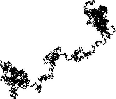
Normal walk on the left, anomalous walk on the right. 10000 steps.
A random walk considers a "walker" which starts somewhere, and takes steps in a random direction. In some cases the steps can be of random length as well. The random walk can take place in a plane, along a line, or in higher dimensions. The simplest random walk considers a walker that takes steps of length 1 to the left or right along a line. More complicated random walks can include fancier considerations, such as giving each step a velocity (random or fixed), and perhaps allowing the random walker to pause for random amounts of time in between the steps.
In the limit as the step length goes to zero and the time between steps goes to zero, the random walker typically exhibits a form of Brownian motion. In the work we do at CNLD, we study random walks that take place in experiments where the individual steps can be seen, and thus the motion is not Brownian motion.
In most cases, a whole group of random walkers spread out in a way called normal diffusion, which is what you probably think of when you think of diffusion. This is what you see if you put dye into a glass of water. The cases where normal diffusion does not occur are called anomalous diffusion, which is what our research is about.
Why might anomalous diffusion occur? If you're stirring the glass of water whenyou put dye in it, you can imagine the dye might spread out differently. Why is this important? In real life, factory smokestacks can dump pollution into the air, which definitely is moving around in complicated ways. Oil tankers spill oil into the ocean, where the motion of the water determines how the oil spreads (rather than just Brownian motion).
This is the theorem that says that "most" random walks spread out like normal diffusion. Normal diffusion is mathematically defined as the variance of a group of random walkers growing linearly in time:
variance = (diffusion constant) * time
The variance is sort of a typical size of the blob of random walkers, and is mathematically defined as the (average of the squares of the distance moved by a random walkers) minus (square of the average of the distance moved by random walkers). The diffusion constant is the rate at which the variance grows. If you put food coloring into water, it spreads out faster (large diffusion constant) compared to putting food coloring into syrup (small diffusion constant).
The Central Limit Theorem says that for most random walks, the details of the random walk only change the diffusion constant, but otherwise the behavior is given by the equation above. For example, a reasonable guess would be that if a random walker takes one step every second, that the diffusion constant would depend on the size of the step. For cases where the step size is random, the diffusion constant actually depends on the average squared step size rather than the average step size. Also, if the random walker takes one step every two seconds, it is reasonable to guess that the diffusion constant would be smaller, and this is correct.
The actual formula for the diffusion constant is D=< L^2 >/T. The meaning of < L^2 > is the average of the square of the step size, and T stands for the average time between each step.
Why is the Central Limit Theorem important? There are many possible ways to have a random step size that will have the same value for < L^2 >, and thus will have the same observable behavior -- the same diffusion constant D. The Central Limit Theorem says that all of these random walks will have the same behavior.
By the way, I'm leaving out a couple technical details: the Central Limit Theorem describes the behavior of a very large number of random walkers as the number of steps they each take gets very large. Small numbers of random walkers do not obey the Central Limit Theorem, nor do random walkers that have not been moving for a long time.
What happens when < L^2 > is infinite? This can happen for certain random walks known as Lévy flights. In this case, the diffusion constant D becomes infinite. At first glance it may appear paradoxical to consider random walks with an infinite average square step size; after all, each step must be of some finite length. An infinite average square step size only means that while long steps are rare, they are not so rare that this average term < L^2 > is finite.
For example, consider a case where a step of length N occurs with a probability proportional to 1/N^2, with N being integers from 1 to infinity. The probability of taking any given step is calculatable, and because the sum of numbers 1/N^2 from 1 to infinity is finite, this is a reasonable choice for a way to take steps of random length -- the total probability can be made to add to 1.
However, consider the average square step size: this is the sum from 1 to infinity of (1/N^2)*(N^2) which is infinite. Thus this type of random walk is of a type not considered by the Central Limit Theorem.
Again I have skipped over some details, but the basic idea is correct. If you consider random walks where the walker goes to the left or to the right, the steps to the left can be considered as steps of a negative length. Of course, the square of a step of negative length is positive and thus a similar argument as above still is correct.
The two pictures at the top of this page are a normal random walk and a Lévy flight. Each walk has a random step length. In the normal case (left, top of this page) the probability of a long step is proportional to L^(-3.8). In the Lévy flight case the probability of a long step is proportional to L^(-2.2), which is more probable than the normal case.
If you follow a normal random walk for a very long time, you start seeing "normal" behavior -- the small steps cannot be seen, and the overall motion is determined by the average affect of all of the steps. For a Lévy flight, the overall position is nearly completely determined by the long, rare steps -- the "flights" -- and thus there is no averaging out of the individual steps.
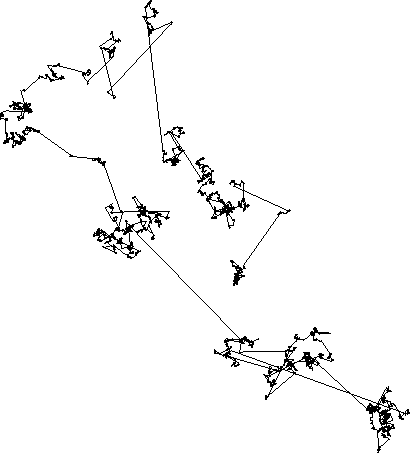
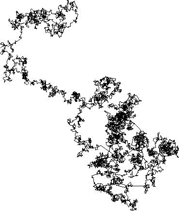
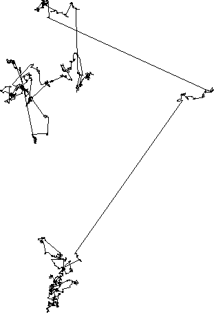
At the top of this page are the normal and Lévy walks for 10000 steps. Those same walks, followed for 100000 steps, are shown here:
Cases with Lévy flights lead to anomalous diffusion: the variance grows faster than linearly in time. In fact, mathematically we write:
variance ~ (time)^gamma
The exponent gamma is equal to one for the normal diffusion case. For Lévy flights, gamma is larger than one (but typically smaller than two). Gamma larger than one is called superdiffusion. Gamma=2 corresponds to "ballistic" motion, such as the particles of a bomb which is exploding. This is the case where all random walkers are moving away from each other at a constant rate.
In some cases, gamma is less than one, called subdiffusion. This corresponds to cases where the average time between steps, called T in the second section, becomes infinite. This can happen in a similar way to the discussion in the previous section. For example, if a pause of duration N occurs with a probability proportional to 1/N^2, the sum which gives the average pause time is a sum of terms like (1/N^2)*N which is the harmonic series, and the sum diverges.
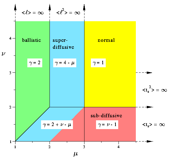
All of this discussion can be summarized in a phase diagram showing how the different behaviors of the step lengths and pause times leads to different forms of diffusion. This phase diagram necessarily depends on some technical details of the random walk.
The horizonal axis of the phase diagram depends on the variable mu, characterizing how the step length distribution is shaped. The meaning of mu is that steps of length L have a probability proportional to L^(-mu). In the example above, mu = 2.
The vertical axis of the phase diagram depends on nu, which characterizes the pauses. Again, the meaning is that pauses of duration t have a probability proportional to t^(-nu). In the example above, nu = 2.
The various shaded regions indicate the type of behavior you would observe given the behavior of the random steps and pauses. The formulae shown for gamma give the exact value of gamma which occurs in each region.
We do work in a rotating annulus where we find random walks. We follow small particles made from chopped up crayons. The particles get trapped in vortices for random amounts of time, acting like the pauses described above. When they leave the vortices they are carried for long distances in jets for random distances, leading to a random walk of random step sizes. We have studied cases where both the pauses and step lengths can lead to anomalous diffusion. In all cases studied, we found either normal diffusion or superdiffusion.
 Click here to see the experimental work.
This work is contained in a paper which has been published in Physica D, volume 97, October 1 1996 (pages 291-310).