Eric Weeks
- personal pages - research
- time series analysis
My Adventures in Chaotic Time Series Analysis |
weeks@physics.emory.edu |
Eric Weeks
- personal pages - research
- time series analysis
My Adventures in Chaotic Time Series Analysis |
weeks@physics.emory.edu |
A0. Links and related information
For an explanation of what these pages are all about, select topic 1 above.
This page: top | lorenz | rossler | henon | expt: periodic | qperiodic-2 | qperiodic-3 | chaotic | bottom
![]()
For a Poincaré section, take an attractor and an arbitrary plane which cuts the attractor into two pieces. The orbits which comprise the attractor cross the plane many times. Plot the intersections of the orbits and the Poincaré plane, although only plot the intersections which occur in one direction (crossing from the "bottom" side to the "top" side for example). This is the Poincaré section, which can reveal structure of the attractor.
Another sort of Poincaré section is when you consider a natural period of the attractor (say, from the fundamental frequency which you could find using a power spectrum).
Brief description of software: I wrote a program called poincare to handle all of this. Click here for more information about this program, including source code.
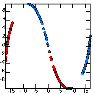
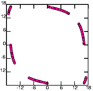
LEFT:
cat 3d.lorenz | poincare -PM3 -d2 -Vn -0.965926 1.032913 -0.008819 |
psdraw -S 10 10 -Cc 0.15 -A > ponlor4.ps
RIGHT:
cat 3d.lorenz | poincare -M3 -d2 -Vn -0.965926 1.032913 -0.008819 | awk '{print $1}' | poincare -om2
I determined the Poincaré plane by studying the 3-D attractor; in the left-hand 3-D picture, the plane is perpendicular to the page and runs through the lower-left corner and the upper-right corner. I determined the plane by the command echo -1 1 0 | rotate -t -15 -p -15 -BC, to get the normal vector to the plane. Note that for the picture above left points are considered which cross in either direction: red are crossing in one direction, blue in the opposite. Both types of points are used for the map (at right).
The Poincaré section above left can be used to construct a 1-D map which is shown above right. Take the x-coordinate of the map; plot x_n and x_n+1 to get the map.
There are six distinct regions which can be seen:
Thus, the regions map A--> EF, B--> C, C--> AB, D--> EF, E--> D, F--> AB. The fact that some regions map onto more than one region implies stretching; the fact that multiple regions map onto one region implies folding.
This is all points intersecting the xy-plane; no other cuts appeared to give any more useful information than this one.
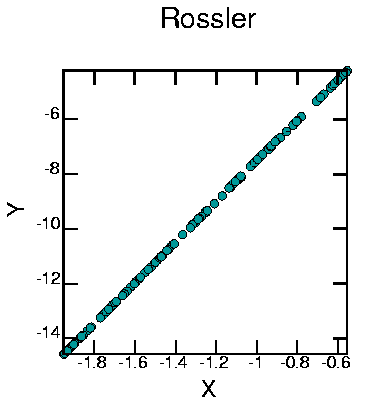
I took the x-coordinate of this graph, and graphed successive values against each other:
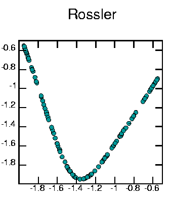
To make this I used: cat 3d.rossler | poincare -VM3 -n 0 0 1 | awk '{print $1}' | poincare -om2 | psdraw -T "Rossler" -S 10 10 -X -2.0 -0.5 -2.0 -0.5 -c0.15 -f 0 153 153 -A > ponros1.ps
Thus, the dynamics of the Rössler attractor can be captured by this one-dimensional map. This map shows stretching (small portions are stretched onto larger portions) and folding (the map has no unique inverse). Recall that the equation describing the Rössler attractor are 3-dimensional; this shows that the dynamics that actually take place can be represented in a 1-dimensional way.
This page:
top |
lorenz |
rossler |
henon |
expt: periodic |
qperiodic-2 |
qperiodic-3 |
chaotic |
bottom
Hénon:
time series
|
power spectrum
|
mutual information
|
attractor
|
attractor 3D
|
autocorrelation
|
poincare
|
1-D maps
I'm not sure what a Poincaré section for the Henon map would be.
Poincaré sections are really intended for data which is in the form
of a continuous orbit; a Poincaré section transforms such data into
a map-like form. The Henon data are already in a map-like form.
This page:
top |
lorenz |
rossler |
henon |
expt: periodic |
qperiodic-2 |
qperiodic-3 |
chaotic |
bottom
Experimental/periodic:
time series
|
power spectrum
|
mutual information
|
attractor
|
attractor 3D
|
autocorrelation
|
poincare
|
1-D maps
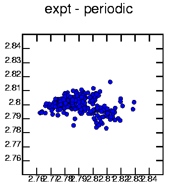
Plotting the attractor in 3 dimensions and taking the xy plane as the Poincaré plane produces the above plot. The scatter in this plot is due to the experimental noise.
This page:
top |
lorenz |
rossler |
henon |
expt: periodic |
qperiodic-2 |
qperiodic-3 |
chaotic |
bottom
Experimental/quasiperiodic-2:
time series
|
power spectrum
|
mutual information
|
attractor
|
attractor 3D
|
autocorrelation
|
poincare
|
1-D maps
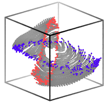
Red points are crossing towards you, blue away from you.
To make this 3-D plot took some work. Here's what I did:
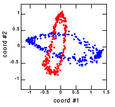
Consider the blue points (points crossing in the direction into the page). Stretch them so that they roughly form a circle. Calculate the angle theta each point makes (with respect to the origin). Graph theta_n -vs- theta_n+1. This results in a nice 1-D map which shows that this is deterministic data:
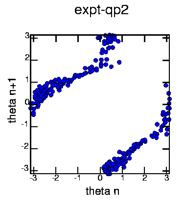
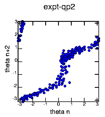
Thus, every second time the Poincaré plane is intersected, the orbit has rotated slightly (generally moving backwards). This map is noisy, but clearly appears to be invertible (that is, each theta_n+2 has a unique theta_n corresponding to it). It has some stretching (angles near theta=0 and theta=pi are mapped to several different values) but overall the map does not appear to be chaotic. Of course, I didn't expect that it would be.
This page:
top |
lorenz |
rossler |
henon |
expt: periodic |
qperiodic-2 |
qperiodic-3 |
chaotic |
bottom
Experimental/quasiperiodic-3:
time series
|
power spectrum
|
mutual information
|
attractor
|
attractor 3D
|
autocorrelation
|
poincare
|
1-D maps
This attractor looks like a tube with a little bit of fuzz inside
it; in the picture below (left), we are looking down the length of the
tube.
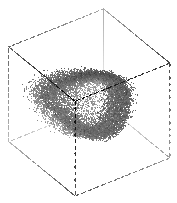
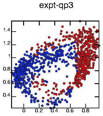
I took a Poincaré plane that cuts this tube parallel to the page, going through the center of the attractor (this plane is perpendicular to the axis of the tube); this is shown in the second picture above.
This was made with:
cat 3d.026 | poincare -n 0.671 0.574 0.470 -d0 -VM3 -x 3.6 3.6 3.6 |
   awk '{print $1,$2,1,0,0}' > datablah

cat 3d.026 | poincare -n 0.671 0.574 0.470 -d1 -VM3 -x 3.6 3.6 3.6 |
   awk '{print $1,$2,0,0.2,1}' > > datablah

psdraw -S 10 10 -T "expt-qp3" -Cc0.12 -f 0 0 255 -A datablah > ponqp3a.ps
Red points are coming out of the page, blue into the page. Looks kinda messy. I took a different Poincaré plane, one that cuts this tube in half lengthwise (parallel to the axis of the tube):
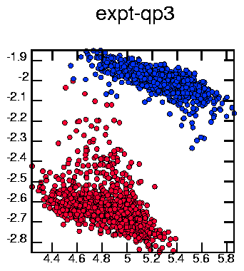
Made with the commands: cat 3d.026 | poincare -Pn -0.470 0.574 0.671 -d2 -VM3 -x 3.6 3.6 3.6 | psdraw -S 10 10 -T "expt-qp3" -Cc0.12 -f 0 0 255 -A > ponqp3b.ps
I then tried a different sort of Poincaré section; I strobed the data every 6.1 seconds (this being the period corresponding to a large peak in the power spectrum). I then graphed the X (red), Y (green), and Z (blue) components, below:
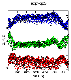
Apparently the data is doing something strange at the beginning and end; this is not suprising as this comes from an experiment, and perhaps the parameters were drifting slightly from beginning to end. Most likely the temperature was changing slightly. I tried redoing the above Poincaré sections using the steady data in the middle, but nothing interesting turned up.
This page:
top |
lorenz |
rossler |
henon |
expt: periodic |
qperiodic-2 |
qperiodic-3 |
chaotic |
bottom
Experimental/chaotic:
time series
|
power spectrum
|
mutual information
|
attractor
|
attractor 3D
|
autocorrelation
|
poincare
|
1-D maps
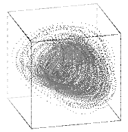
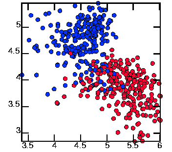
The Poincaré plane is taken perpendicular to the page, with the normal vector pointing roughly at 75 degrees from the horizonal (in the (1,4) direction). I used the command: cat 3d.042 | poincare -d2 -PVM3 -n 1.365926 -3.670249 1.017 -x 3.8 3.8 3.8 | psdraw -S 10 10 -Cc0.15 -f 0 0 255 -T "expt - chaotic" -A > poncha2.ps
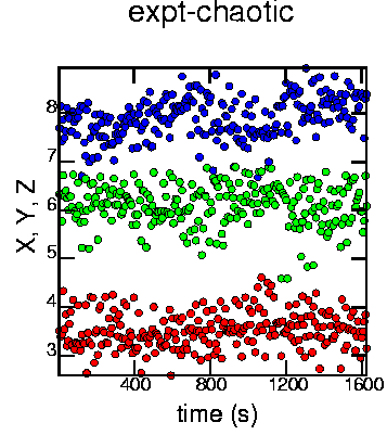
Similar to the graph for the qp-3 data, this is a Poincaré section based on strobing at a period of 6.535 s (derived from the power spectrum). Plotted are the X (red), Y (green), and Z (blue) coordinates (they have been offset slightly from each other). I can't see much of any pattern.
![]()
So far the analysis has given me several different times. From the Fourier transform I have certain characteristic periods. From the mutual information calculation I have the first minimum. I also have the autocorrelation first zero-crossing.
Note that all times are in natural units (seconds for experimental data, iterations for Hénon map, the time step of the equations for the Rössler and Lorenz systems). Links in the table will take you to the appropriate location where the information was found.
 Previous page: Autocorrelation
 Next page: Another way to determine 1-D maps from data.
This page: top | lorenz | rossler | henon | expt: periodic | qperiodic-2 | qperiodic-3 | chaotic | bottom
![]()